第 6 章 BAS案例一:多杆机构优化问题
说明:由于自身专业知识局限,在整理转述各位研究者或贡献者所提供的材料时,我可能无法准确地表达出对应领域的知识要点。避免言多必失,我仅仅做简要的翻译或者是介绍。对于读者而言,如果觉得并不能解你之疾,或没有挠到痒处,建议直接和对应的作者联系。对于贡献者而言,如果我表述有误,欢迎提出建议,或者在github上pull request。
由群友莫小娟博士研究生提供案例。
由于案例均为各位热心的同学提供,均为自己的研究。因此,希望大家要引用其中的结果时,可以引用对应同学的文章。此外,也请大家转载时注明来源。
6.1 背景
6.1.1 四连杆机构(Four-bar linkage mechanism)
四连杆机构如图6.1所示:
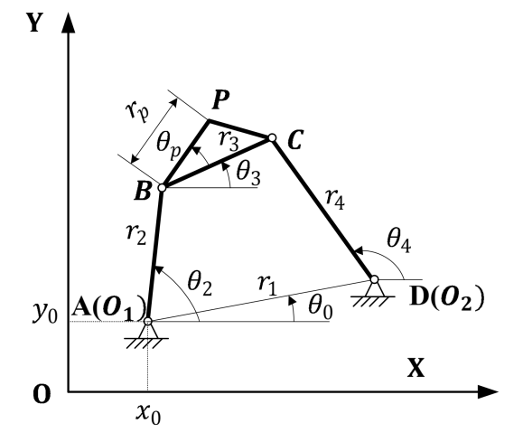
图 6.1: 四连杆机构示意
基于闭环矢量方程,推导出节点位置。推导过程如式(6.1)至式(6.4):
\[\begin{equation} \mathbf{\text{Loop:}} r_1e^{i\theta_0} + r_4e^{i\theta_4} - r_2e^{i\theta_2} -r_3e^{i\theta_3} = 0\\ \tag{6.1} \end{equation}\]
\[\begin{equation} \begin{cases} r_1cos(\theta_0) + r_4cos(\theta_4)-r_2cos(\theta_2)-r_3cos(\theta_3)=0 \\ r_1sin(\theta_0) + r_4sin(\theta_4)-r_2sin(\theta_2)-r_3sin(\theta_3)=0 \end{cases} \tag{6.2} \end{equation}\]
\[\begin{equation} \begin{split} &\theta_3 =2atan(\frac{-A\pm\sqrt{2}{A^2-4BC}}{2B})+\theta_0\\ &A = cos(\theta_2 - \theta_0)-K_1+K_2cos(\theta_2-\theta_0)+K_3\\ &B = -2sin(\theta_2-\theta_0), F=K_1+(K_2-1)cos(\theta_2-\theta_0)+K_3\\ &K_1 = r_1/r_2,K_2=r_1/r_3,K_3=(r_4^2-r_1^2-r_2^2-r_3^2)/(2r_2r_3)\\ \end{split} \tag{6.3} \end{equation}\]
\[\begin{equation} \begin{cases} x_p=x_0+r_2cos(\theta_2)+r_pcos(\theta_3+\theta_p) \\ y_p=y_0+r_2sin(\theta_2)+r_psin(\theta_3+\theta_p) \end{cases} \tag{6.4} \end{equation}\]
6.1.2 六连杆机构(Stephenson III Six-bar linkage mechanism)
六连杆机构如图6.2所示:
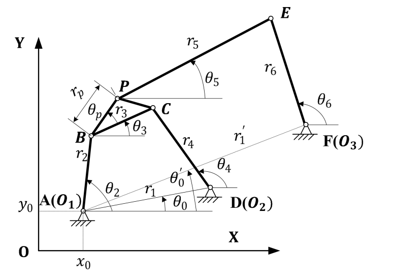
图 6.2: 六连杆机构示意
基于闭环矢量方程,推导出节点位置和外部链接角度。推导过程如式(6.5)至式(6.6):
\[\begin{equation} \begin{split} &\mathbf{\text{Loop1:}} r_1e^{i\theta_0} + r_4e^{i\theta_4} - r_2e^{i\theta_2} -r_3e^{i\theta_3} = 0\\ &\mathbf{\text{Loop2:}} r_1'e^{i\theta_0'} + r_6e^{i\theta_6} - r_2e^{i\theta_2} -r_pe^{i(\theta_3+\theta_p)}-r_5e^{i\theta_5} = 0\\ \end{split} \tag{6.5} \end{equation}\]
\[\begin{equation} \begin{split} \text{Loop1:}\\ &\alpha = r_2cos(\theta_2) - r_1cos(\theta_0), \beta = r_2sin(\theta_2)-r_1sin(\theta_0) \\ &\gamma = (r_4^2+\alpha^2+\beta^2-r_3^2)/(2r_4),\lambda=atan2(\alpha,\beta)\\ &\theta_4 = atan(cos(\lambda)\gamma/\beta,\{1-(cos(\lambda)\gamma/\beta)^2\}^{1/2})-\lambda\\ &\theta_3=atan2(r_4sin(\theta_4)-\beta,r_4cos(\theta_4)-\alpha)\\ \text{Loop2:}\\ &\alpha_1 = r_2cos(\theta_2)+r_pcos(\theta_3+\theta_p)-r_6cos(\theta_6)\\ &\beta_1=r_2sin(\theta_2)+r_psin(\theta_3+\theta_p)-r_6sin(\theta_6)\\ &\gamma_1=(r_6^2+\alpha_1^2+\beta_1^2-r_5^2)/(2r_6),\lambda_1=atan2(\alpha_1,\beta_1)\\ &\theta_6=atan2(cos(\lambda)\gamma_1/\beta_1,-\{1-(cos(\lambda_1)\gamma_1/\beta_1)^{2}\}^{1/2}) - \lambda_1\\ &\theta_5 = atan2(r_6sin(\theta_6)-\beta_1,r_6cos(\theta_6)-\alpha_1) \end{split} \tag{6.6} \end{equation}\]
于是,可以得到节点位置如式(6.7):
\[\begin{equation} \begin{cases} x_A = x_0,y_A = y_0 \\ x_D = x_0+r_1cos(\theta_0),y_D = y_0+r_1sin(\theta_0)\\ x_F = x_0+r_1'cos(\theta_0'),x_F = x_0 + r_1'sin(\theta_0')\\ x_p = x_0 + r_2cos(\theta_2) + r_pcos(\theta_3+\theta_p)\\ y_P = y_0 + r_2sin(\theta_2)+r_Psin(\theta_3+\theta_p)\\ \end{cases} \tag{6.7} \end{equation}\]
6.2 优化问题
6.2.1 四连杆机构
四杆机构的优化问题可以用式(6.8)表示。
\[\begin{equation} \begin{split} \text{min } &\sum_{i=1}^N[(P_{Xd}^i-P_X^i)^2+(P_{Yd}^i-P_Y^i)^2]+M_1h_1(x)+M_2h_2(x)\\ \text{where } & x_i\in [l_{min}^i,l_{max}^i] \quad \forall x_i \in X,\\ &X=[r_1,r_2,r_3,r_4,r_p,\theta_p,\theta_0,x_0,y_0,\theta_2^1,\cdots,\theta_2^N]\\ \end{split} \tag{6.8} \end{equation}\]
其中,
\[\begin{equation} h_1(x) = \begin{cases} 1, & \text{the Grashof condition false}\\ 0, & \text{the Grashof condition true} \end{cases} \tag{6.9} \end{equation}\]
\[\begin{equation} h_2(x) = \begin{cases} 1, & \text{the sequence condition of the crank angle false}\\ 0, & \text{the sequence condition of the crank angle true} \end{cases} \tag{6.10} \end{equation}\]
\(h_1(X)\) 和 \(h_2(X)\) 分别用于评估曲柄存在条件(Grashof Condition)以及曲柄角度(顺时针或逆时针)的顺序情况。\(M_1\) 和 \(M_2\)分别是对应的惩罚系数。\(X\) 为设计参数。
6.2.2 六连杆机构
\[\begin{equation} \begin{split} \text{min } &\sum_{i=1}^N[(P_{Xd}^i-P_X^i)^2+(P_{Yd}^i-P_Y^i)^2]+\sum_{i=1}^M[(\theta_{6d}^i-\theta_6^i)^2]\\ &+M_1h_1(x)+M_2h_2(x)+M_3h_3(X)\\ \text{where } & x_i\in [l_{min}^i,l_{max}^i] \quad \forall x_i \in X,\\ &X=[r_1,r_2,r_3,r_4,r_5,r_6,r_p,\theta_p,\theta_0,x_0,y_0,\theta_2^1,\cdots,\theta_2^N]\\ \end{split} \tag{6.11} \end{equation}\]
其中,\(h_1(X)\) 与 \(h_2(X)\) 同式(6.9)与(6.10), \(h_3(X)\)如式(6.12):
\[\begin{equation} h_3(x) = \begin{cases} 1, & \text{non-violation of transmission angle false}\\ 0, & \text{non-violation of transmission angle true} \end{cases} \tag{6.12} \end{equation}\]
\(h_3(X)\) 所表示的是,是否没有违背传动角(超过20°)的约束。同样地,\(M_3\) 为对应的惩罚系数。
6.3 优化理论
案例所使用的算法是标准化的群体天牛算法。有意思的是,此处群体天牛算法,和rBAS包的BSASoptim的算法极为类似。这也说明,加入群体智能策略,会使得BAS对于复杂问题寻优能力增强。
联系在于:此案例使用的群体天牛,是在每回合,对于天牛探索方向数的提升。即,每回合生成多个随机的方向,在这些方向上,派出天牛进行试探。这点和BSAS保持一致,可以理解为,如果天牛不止有一对须,而是有多对,那每回合探索的方向也会有多个。大致的原理如式(6.13):
\[\begin{equation} \begin{split} x_{ri} &= x_{t} + d^t\overrightarrow{b_i}, \quad i = 1,\cdots,q\\ x_{li} &= x_{t} - d^t\overrightarrow{b_i}, \\ x_{ti} &= x_{t-1} - \delta^t\overrightarrow{b_i}sign(f(x_{ri})-f(x_{li})) \end{split} \tag{6.13} \end{equation}\]
区别在于:并未使用基于结果反馈的步长调节策略。
对于轨迹优化问题,莫小娟同学给出的参数建议是,\(d_0 = 0.10,\delta_0=0.05,c_1=0.9998,c_2=0.5,q=40,T_{max}=50000\)。部分同学可能看过手册的2节,对于步长\(d\)和须到质心距离\(\delta\)的更新,即式(2.6)中有所提及。此处,参数的含义如式(6.14)所示。部分参数与式(2.6)类同,也有同名但含义冲突的,大家复现时需要注意这些地方。
\[\begin{equation} \begin{split} d^t &= c_1d^{t-1}\\ \delta^t&=c_2 d^t\\ \end{split} \tag{6.14} \end{equation}\]
6.4 优化结果
此处,莫小娟同学提供了8个案例,并且与其他的经典算法(指多杆机构优化问题中多用的算法)进行了优化效果的对比。
6.4.1 Case1 无规定时间内轨迹生成(Path generation without prescribed timing)
本案例是四杆机构的路径(6个点)在一条垂直的线上(没有规定时间)。通过式(6.8)计算得到误差。
设计参数为:
\[ X = [r_1,r_2,r_3,r_4,r_p,\theta_p,\theta_0,x_0,y_0,\theta_2^1,\cdots,\theta_2^6] \] 目标点坐标:
\[ \{C_d^i\} = \{(20,20),(20,25),(20,30),(20,40),(20,45)\} \]
参数约束:
\[ r_1,r_2,r_3,r_4\in[0,60]\quad r_p,x_0,y_0\in[-60,60]\quad \theta_0,\theta_1,\cdots,\theta_2^6,\theta_p\in[0,2\pi] \] 算法参数为 \(d_0 = 0.10,\delta_0=0.05,c_1=0.9998,c_2=0.5,q=40,T_{max}=50000\),动画结果如图6.3。
图 6.3: 四杆机构轨迹生成
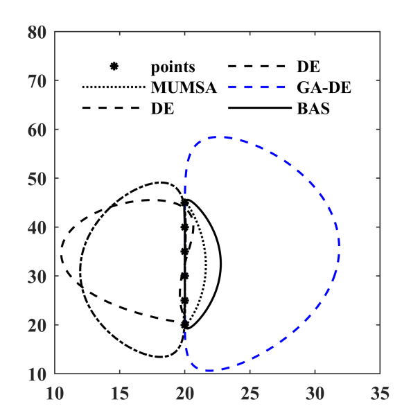
图 6.4: 各算法优化轨迹
| MUMSA | GA | DE | GA.DE | BAS | |
|---|---|---|---|---|---|
| \(r_1\) | 31.788264 | 28.771330 | 35.020740 | 13.2516000 | 19.4920810 |
| \(r_2\) | 8.204647 | 5.000000 | 6.404196 | 5.9407800 | 6.2644716 |
| \(r_3\) | 24.932131 | 35.365480 | 31.607220 | 58.3118000 | 20.1001631 |
| \(r_4\) | 31.385926 | 59.136810 | 50.599490 | 53.7207000 | 19.0219161 |
| \(r_p\) | 37.108246 | 14.850370 | 46.461261 | 61.3011560 | 39.8538048 |
| \(\theta_p\) | 0.398977 | 1.570796 | 1.106544 | -1.3002600 | 0.3679660 |
| \(\theta_0\) | 4.015959 | 5.287474 | 0.000000 | 0.1960760 | 4.4245619 |
| \(x_0\) | -6.366519 | 29.913290 | 60.000000 | -35.3621000 | -13.0300715 |
| \(y_0\) | 56.836760 | 32.602280 | 18.077910 | 36.7704000 | 51.1796666 |
| \(\theta_2^1\) | 1.366547 | 6.283185 | 6.283185 | 1.6601500 | 5.9699819 |
| \(\theta_2^2\) | 2.330773 | 0.318205 | 0.264935 | 2.0468400 | 0.4554995 |
| \(\theta_2^3\) | 2.871039 | 0.638520 | 0.500377 | 2.4281100 | 1.0202707 |
| \(\theta_2^4\) | 3.394591 | 0.979950 | 0.735321 | 2.8090100 | 1.5550696 |
| \(\theta_2^5\) | 3.970960 | 1.412732 | 0.996529 | 3.1900900 | 2.1117409 |
| \(\theta_2^6\) | 4.963490 | 2.076254 | 1.333549 | 3.5737900 | 2.8839248 |
| \(Error\) | 0.002057 | 1.101697 | 0.122738 | 0.0000172 | 0.0000124 |
6.4.2 Case2 有规定时间的轨迹生成(with prescribed timing)
本案例四杆机构的路径为5个没有对齐的点(规定时间)。通过式(6.8)计算得到误差。
设计参数为:
\[ X = [r_1,r_2,r_3,r_4,r_p,\theta_p] \] 目标点坐标:
\[\begin{align} &\{C_d^i\} = \{(3,3),(2.759,3.363),(2.759,3.363),(1.890,3.862),(1.355,3.943)\} \notag \\ &\{\theta_2^1,\theta_2^2,\theta_2^3,\theta_2^4,\theta_2^5\}=\{\pi/6,\pi/4,\pi/3,5\pi/12,\pi/2\} \notag \\ \end{align}\]
参数约束:
\[ r_1,r_2,r_3,r_4\in[0,5]\quad r_p\in[-5,5]\quad \theta_p\in[0,2\pi] \]
算法参数为 \(d_0 = 0.10,\delta_0=0.05,c_1=0.9998,c_2=0.5,q=40,T_{max}=10000\),动画结果如图6.5。
图 6.5: case2四杆机构轨迹生成
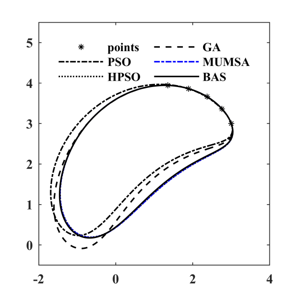
图 6.6: 各算法优化轨迹
| PSO | HPSO | GA | MUMSA | BAS | |
|---|---|---|---|---|---|
| \(r_1\) | 3.0576200 | 3.7877200 | 3.0630424 | 3.7732686 | 3.7135255 |
| \(r_2\) | 1.8618400 | 1.9984200 | 1.9959624 | 2.0000040 | 1.9978745 |
| \(r_3\) | 3.8459100 | 4.1331300 | 3.3058230 | 4.1169710 | 4.0469527 |
| \(r_4\) | 2.9706300 | 2.7451300 | 2.5247060 | 2.7461567 | 2.7192391 |
| \(r_p\) | 2.4968270 | 2.3697220 | 2.3721479 | 2.3684374 | 2.3702974 |
| \(\theta_p\) | 0.7243557 | 0.7841479 | 0.8044176 | 0.7831567 | 0.7865371 |
| \(Error\) | 0.0005860 | 0.0009860 | 0.0000018 | 0.0000018 | 0.0000007 |
6.4.3 Case3 规定时间内路径生成(Path generation with prescribed timing)
本案例四杆机构需要在规定时间通过一个闭环。通过式(6.8)计算得到误差。
设计参数为:
\[ X = [r_1,r_2,r_3,r_4,r_p,\theta_p,\theta_0,x_0,y_0,\theta_2^1,\cdots,\theta_2^6] \]
目标点坐标:
\[\begin{align} \{C_d^i\} = \{&(0.5,1.1),(0.4,1.1),(0.3,1.1),(0.2,1.0),(0.1,0.9),(0.05,0.75), \notag \\ &(0.02,0.6),(0,0.5),(0,0.4),(0.03,0.3),(0.1,0.25),(0.15,0.2), \notag\\ &(0.2,0.3),(0.3,0.4),(0.4,0.5),(0.5,0.7),(0.6,0.9),(0.6,1.0)\} \notag\\ \{\theta_2^i\}=\{&\theta_2^1,\theta_2^1+20\cdot i/\pi\},\quad i = 1,\cdots,17 \notag \\ \end{align}\]
参数约束:
\[ r_1,r_2,r_3,r_4\in[0,5]\quad r_p,x_0,y_0\in[-5,5]\quad \theta_0,\theta_2^1,\theta_p\in[0,2\pi] \]
算法参数为 \(d_0 = 0.10,\delta_0=0.05,c_1=0.9998,c_2=0.5,q=8,T_{max}=50000\),动画结果如图6.7。
图 6.7: case3四杆机构轨迹生成
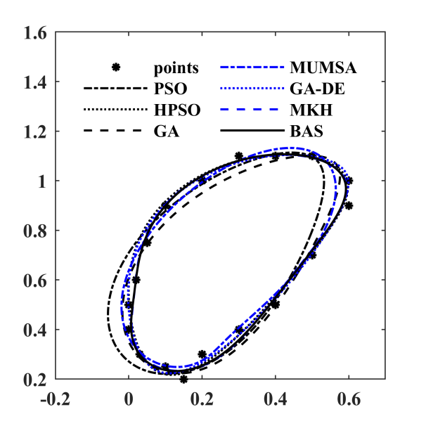
图 6.8: 各算法优化轨迹
| PSO | HPSO | GA | MUMSA | GA.DE | MKH | BAS | |
|---|---|---|---|---|---|---|---|
| \(r_1\) | 2.9261 | 2.8500 | 3.0579 | 4.4538 | 47.4379 | 1.0043 | 1.0542 |
| \(r_2\) | 0.4877 | 0.3700 | 0.2378 | 0.2971 | 0.3248 | 0.4218 | 0.4239 |
| \(r_3\) | 2.9099 | 2.9048 | 4.8290 | 3.9131 | 0.4729 | 0.8782 | 0.9146 |
| \(r_4\) | 2.1503 | 0.5000 | 2.0565 | 0.8494 | 47.3093 | 0.5801 | 0.5989 |
| \(r_p\) | 1.4939 | 1.9737 | 2.0035 | 2.6520 | 0.3413 | 0.5234 | 0.5450 |
| \(\theta_p\) | -0.3325 | 1.0274 | 1.1779 | 2.4647 | -1.2154 | 0.8148 | 0.8227 |
| \(\theta_0\) | 0.7190 | 0.7600 | 1.0022 | 2.7387 | 3.3203 | 0.2929 | 0.2850 |
| \(x_0\) | -0.3846 | 0.9400 | 1.7768 | -1.3092 | 0.5270 | 0.2689 | 0.2677 |
| \(y_0\) | -0.6752 | -1.1712 | -0.6420 | 2.8070 | 0.7239 | 0.1772 | 0.1544 |
| \(\theta_2^1\) | 0.2159 | 0.5134 | 0.2262 | 4.8535 | 3.5123 | 0.8860 | 1.1764 |
| \(Error\) | 0.0492 | 0.0111 | 0.0337 | 0.0196 | 0.0109 | 0.0091 | 0.0090 |
6.4.4 Case4 规定时间路径生成问题
第四个案例同样是一个规定时间的路径生成问题。六个优化点由一个semi-archer弧构成,问题定义如下。
设计参数为:
\[ X = [r_1,r_2,r_3,r_4,r_p,\theta_p,\theta_0,x_0,y_0] \]
目标点坐标:
\[\begin{align} &\{C_d^i\} = \{(0,0),(1.9098,5.8779),(6.60989.5106),(13.09,9.5106),(18.09,5.8779),(20,0)\} \notag \\ &\{\theta_2^1,\theta_2^2,\theta_2^3,\theta_2^4,\theta_2^5\}=\{\pi/6,\pi/3,\pi/2,2\pi/3,5\pi/6,\pi\} \notag \\ \end{align}\]
参数约束:
\[ r_1,r_2,r_3,r_4\in[0,50]\quad r_p,x_0,y_0\in[-50,50]\quad \theta_0,\theta_p\in[0,2\pi] \]
算法参数为 \(d_0 = 0.10,\delta_0=0.05,c_1=0.9997,c_2=0.5,q=40,T_{max}=30000\),动画结果如图6.9。
图 6.9: case4四杆机构轨迹生成
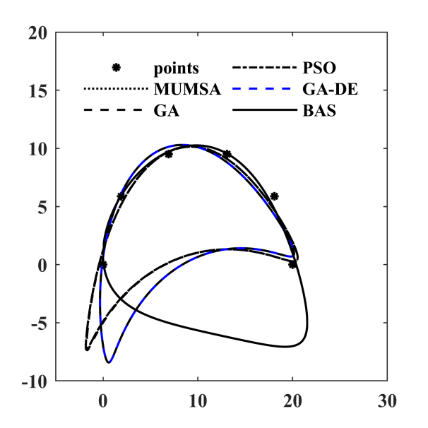
图 6.10: 各算法优化轨迹
| MUMSA | GA | PSO | GA.DE | BAS | |
|---|---|---|---|---|---|
| \(r_1\) | 50.0000000 | 50.0000000 | 50.0000000 | 50.000000 | 47.2345017 |
| \(r_2\) | 5.0000000 | 5.0000000 | 5.0000000 | 5.000000 | 8.8473992 |
| \(r_3\) | 7.0310470 | 6.9700900 | 7.0310200 | 5.905343 | 25.0474709 |
| \(r_4\) | 48.1341830 | 48.1993000 | 48.1342000 | 50.000000 | 50.0000000 |
| \(r_p\) | 21.3533558 | 21.2191204 | 21.3532819 | 18.819312 | 50.0000000 |
| \(\theta_p\) | 0.6517294 | 0.6380060 | 0.6517238 | 0.000000 | 5.7107187 |
| \(\theta_0\) | 0.0428247 | 0.0508453 | 0.0428286 | 0.463633 | 0.8225945 |
| \(x_0\) | 12.1974940 | 12.2377000 | 12.1975000 | 14.373772 | 16.5531171 |
| \(y_0\) | -15.9982030 | -15.8332000 | -15.9981000 | -12.444295 | -48.1473786 |
| \(Error\) | 2.5803500 | 2.5828600 | 2.5803600 | 2.349649 | 0.7863680 |
6.4.5 Case5 规定时间内路径生成问题
这个例子是一个椭圆路径生成问题,没有规定的时间,其中轨迹是由10个点定义的。问题定义如下。
设计参数为:
\[ X = [r_1,r_2,r_3,r_4,r_p,\theta_p,\theta_0,x_0,y_0,\theta_2^1,\cdots,\theta_2^{10}] \]
目标点坐标:
\[\begin{align} \{C_d^i\} = \{&(20,10),(17.66,15.142),(11.736,17.878),(5,16.928),(0.60307,12.736), \notag \\ &(0.60307,7.2638),(5,3.0718),(11.736,2.1215),(17.66,4.8577),(20,0)\}\notag\\ \end{align}\]
参数约束:
\[ r_1,r_2,r_3,r_4\in[0,80]\quad r_p,x_0,y_0\in[-80,80]\quad \theta_0,\theta_2^1,\cdots,\theta_2^{10},\theta_p\in[0,2\pi] \]
算法参数为 \(d_0 = 0.10,\delta_0=0.05,c_1=0.9998,c_2=0.5,q=40,T_{max}=40000\),动画结果如图6.11。
图 6.11: case5四杆机构轨迹生成
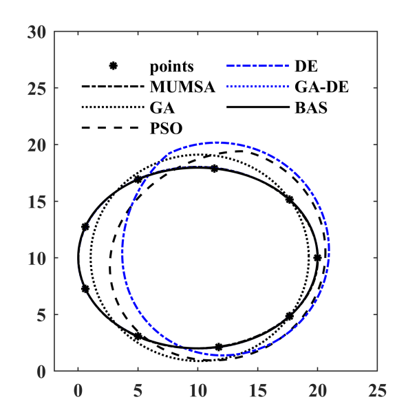
图 6.12: 各算法优化轨迹
| MUMSA | GA | PSO | DE | GA.DE | BAS | |
|---|---|---|---|---|---|---|
| \(r_1\) | 79.5160680 | 79.981513 | 52.535162 | 54.360893 | 80.0000000 | 71.8681225 |
| \(r_2\) | 9.7239730 | 9.109993 | 8.687886 | 8.683351 | 8.4203200 | 9.2618623 |
| \(r_3\) | 45.8425240 | 72.936511 | 36.155078 | 34.318634 | 51.3426000 | 44.4542963 |
| \(r_4\) | 51.4384800 | 80.000000 | 80.000000 | 79.996171 | 42.4532000 | 43.0533508 |
| \(r_p\) | 8.7289390 | 0.000000 | 1.481055 | 1.465250 | 10.6530404 | 8.7820722 |
| \(\theta_p\) | -0.3452264 | 0.000000 | 1.570796 | 1.570669 | 2.6465448 | 1.6362575 |
| \(\theta_0\) | 5.5969445 | 0.026149 | 1.403504 | 2.129650 | 4.2817700 | 1.6011655 |
| \(x_0\) | 2.0211090 | 10.155966 | 11.002124 | 10.954397 | 5.5337200 | 16.7540360 |
| \(y_0\) | 13.2165878 | 10.000000 | 11.095585 | 11.074534 | 0.4771830 | 15.2986682 |
| \(\theta_2^1\) | 0.6376873 | 6.283185 | 6.282619 | 6.283185 | 2.0935000 | 0.1258416 |
| \(\theta_2^2\) | 1.3255329 | 0.600745 | 0.615302 | 0.616731 | 2.8129100 | 0.8167208 |
| \(\theta_2^3\) | 2.0080339 | 1.372812 | 1.305421 | 1.310254 | 3.5160500 | 1.5351326 |
| \(\theta_2^4\) | 2.6955659 | 2.210575 | 2.188053 | 2.193570 | 4.2063800 | 2.1811489 |
| \(\theta_2^5\) | 3.3845794 | 2.862639 | 2.913049 | 2.917170 | 4.8905100 | 2.8753839 |
| \(\theta_2^6\) | 4.0829376 | 3.420547 | 3.499313 | 3.490746 | 5.5739800 | 3.5728072 |
| \(\theta_2^7\) | 4.7984548 | 4.072611 | 4.125586 | 4.132017 | 6.2645800 | 4.2854058 |
| \(\theta_2^8\) | 5.5117056 | 4.910373 | 4.919977 | 4.922075 | 0.6761980 | 5.0016208 |
| \(\theta_2^9\) | 6.2127919 | 5.682440 | 5.685021 | 5.695372 | 1.3830700 | 5.7133417 |
| \(\theta_2^{10}\) | 0.6371866 | 6.283185 | 6.282323 | 6.282970 | 2.0934800 | 0.1258290 |
| \(Error\) | 0.0047000 | 2.281273 | 1.971004 | 1.952326 | 0.0006022 | 0.0004252 |
6.4.6 Case6 六杆机构路径生成
这个案例我也看不懂。大概意思是,六杆问题,在规定时间内让轨迹耦合目标点,并且output link在停顿位置(dwell portion?我翻译不下去了……)保持在一个精确的角度。大家看底下的原文靠谱一点。
“This case is a path and function combined synthesis problem with prescribed timing in which the coupler of six-bar mechanism has to the precision points and its output link has to maintain an accuracy angle in the dwell portion.”
— Xiaojuan Mo
设计参数为:
\[ X = [r_1,r_2,r_3,r_4,r_5,r_6,r_p,\theta_p,r_1',\theta_0,\theta_0',x_0,y_0,\theta_2^1] \]
目标点坐标:
\[\begin{align} \{C_d^i\} = \{&(-0.5424,2.3708),(0.2202,2.9871),(0.9761,3.4633), \notag \\ &(1.0618,36380),(0.8835,3.7226),(0.5629,3.7156),\notag \\ &(0.1744,3.6128),(-0.2338,3.4206),(-0.6315,3.1536), \notag \\ &(-1.0,2.8284),(-1.3251,2.4600),(-1.5922,2.0622), \notag \\ &(-1.7844,1.6539),(-1.8872,1.2654),(-1.8942,0.9448), \notag \\ &(-1.8096,0.7665),(-1.6349,0.8522),(-1.1587,1.6081)\} \notag \\ \{\theta_2^i\} = \{&0,15,40,60,80,100,120,140,160,180,\notag \\ & 200, 220,240,260,280,300,320,345\} \notag \\ & \rightarrow \theta_2^i = \theta_2 + \delta_2^i \notag \\ \end{align}\]
在停顿位置处的输入输出角度的关联如下:
\[\begin{align} &\theta_2^i = \theta_2^1+\{160,180,200,220\}\rightarrow \theta_6^i=210 \notag \\ &\theta_2^i=\theta_2^1+\{345,0,15\} \rightarrow \theta_6^i = 225 \notag \\ \end{align}\]
注意,上述涉及到角度的数值单位均为deg,而非弧度。
算法参数为 \(d_0 = 0.05,\delta_0=0.025,c_1=0.9999,c_2=0.5,q=10,T_{max}=50000\),动画结果如图6.13。
图 6.13: case6六杆机构轨迹生成
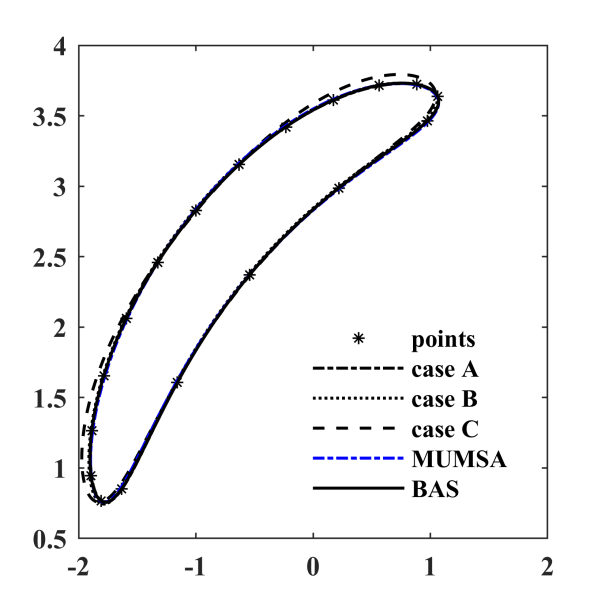
图 6.14: 各算法优化轨迹
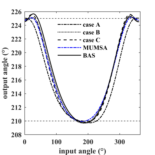
图 6.15: 各算法优化角度
| DE.A | DE.B | DE.C | MUMSA | BAS | |
|---|---|---|---|---|---|
| \(r_1\) | 1.8145 | 1.8065 | 2.0926 | 1.713529 | 1.838058488 |
| \(r_2\) | 0.9911 | 0.9826 | 1.1464 | 0.92602 | 1.006097698 |
| \(r_3\) | 1.9995 | 2.0177 | 1.989 | 1.991373 | 1.997800646 |
| \(r_4\) | 2.0315 | 2.0009 | 1.9727 | 1.848672 | 2.008472163 |
| \(r_5\) | 4.3674 | 5.7769 | 6.6633 | 5.35498 | 6.106586728 |
| \(r_6\) | 2.4924 | 2.5296 | 2.5517 | 2.54979 | 2.551492193 |
| \(r_p\) | 2.8174 | 2.8711 | 2.7178 | 2.975936132 | 2.815041279 |
| \(\theta_p\) | 0.7776 | 0.783712 | 0.845246 | 0.831651258 | 0.78386985 |
| \(\theta_0\) | 6.269879 | 0.011582 | 6.242260827 | 0.067677 | 6.277427755 |
| \(r_1'\) | 4.4158 | 5.2817 | 6.2907 | 4.87374 | 5.63828226 |
| \(\theta_0'\) | 0.235595 | 0.0170309 | 6.18118303 | 0.0967027 | 6.257863894 |
| \(x_0\) | 0.0115 | 0.0415 | -0.2729 | 0.175257 | -0.013849346 |
| \(y_0\) | 0.0157 | -0.0377 | 0.0931 | -0.1187032 | 0.011591976 |
| \(\theta_2^1\) | 0.00052 | 0.003648 | -0.04062 | 6.222361 | 6.281768246 |
| \(Evaluations\) | 53310 | 93405 | 93405 | 93405 | 50000 |
| \(Error\) | 0.000250876 | 0.005653158 | 0.03537533 | 0.0014 | 0.000195212659 |
6.4.7 Case7 无规定时间的路径生成
本案例为一个’8’型路径生成问题,轨迹由12个点规定。
设计参数为:
\[ X = [r_1,r_2,r_3,r_4,r_p,\theta_p,\theta_0,x_0,y_0,\theta_2^1,\cdots,\theta_2^{12}] \]
目标点坐标:
\[\begin{align} \{C_d^i\} = \{&(4.15,2.21),(4.50,2.18),(4.53,1.83),(4.13,1.68),(3.67,1.58),(2.96,1.33), \notag \\ &(2.67,1.06),(2.63,0.82),(2.92,0.81),(3.23,1.07),(3.49,1.45),(3.76,1.87)\}\notag\\ \end{align}\]
参数约束:
\[\begin{align} &r_1\in[0,5]\quad r_2,r_3,r_4\in[0,10] \quad r_p\in[0,14],\notag \\ &x_0,y_0\in[-80,80]\quad \theta_0,\theta_2^1,\cdots,\theta_2^{12},\theta_p\in[0,2\pi] \notag \\ \end{align}\]
算法参数为 \(d_0 = 0.05,\delta_0=0.025,c_1=0.9995,c_2=0.5,q=40,T_{max}=20000\),动画结果如图6.16。
图 6.16: case7机构轨迹生成
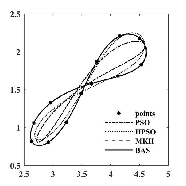
图 6.17: 各算法优化轨迹
| PSO | HPSO | MKH | BAS | |
|---|---|---|---|---|
| \(r_1\) | 4.550300 | 4.535900 | 2.8764500 | 2.8162769 |
| \(r_2\) | 1.101300 | 1.113300 | 1.1464400 | 1.1382629 |
| \(r_3\) | 3.955800 | 14.738100 | 4.4077300 | 4.0509922 |
| \(r_4\) | 3.933000 | 16.801700 | 4.7571300 | 4.1957758 |
| \(r_p\) | 3.941572 | 3.941866 | 2.6665746 | 2.6682801 |
| \(\theta_p\) | -0.539171 | -1.521104 | -1.1363513 | 5.1910788 |
| \(\theta_0\) | 0.000000 | 0.000000 | 0.1650200 | 0.2070603 |
| \(x_0\) | 0.000000 | 0.000000 | 1.1426500 | 1.1226995 |
| \(y_0\) | 0.000000 | 0.000000 | 0.4823700 | 0.5246662 |
| \(\theta_2^1\) | -0.201400 | -0.181600 | -0.3139900 | 6.1191060 |
| \(Error\) | 0.171600 | 0.096400 | 0.0001597 | 0.0000994 |
6.4.8 Case8 无规定时间的路径生成
本案例为一个叶形路径生成问题(无规定时间),轨迹由25个点规定。
设计参数为:
\[ X = [r_1,r_2,r_3,r_4,r_p,\theta_p,\theta_0,x_0,y_0,\theta_2^1,\cdots,\theta_2^{25}] \]
目标点坐标:
\[\begin{align} \{C_d^i\} = \{&(7.03,5.99),(6.95,5.45),(6.77,5.03),(6.4,4.6),(5.91,4.03), \notag \\ &(5.43,3.56),(4.93,2.94),(4.67,2.6),(4.38,2.2),(4.04,1.67),\notag \\ &(3.76,1.22),(3.76,1.97),(3.76,2.78),(3.76,3.56),(3.76,4.34), \notag \\ &(3.76,4.91),(3.76,5.47),(3.8,5.98),(4.07,6.4),(4.53,6.75), \notag \\ &(5.07,6.85),(5.05,6.84),(5.89,6.83),(6.41,6.8),(6.92,6.58)\} \notag \\ \end{align}\]
参数约束:
\[ r_1,r_2,r_3,r_4\in[0,5]\quad r_p,x_0,y_0\in[-5,5] \quad \theta_0,\theta_2^1,\cdots,\theta_2^{25},\theta_p\in[0,2\pi] \]
算法参数为 \(d_0 = 0.05,\delta_0=0.025,c_1=0.99975,c_2=0.5,q=40,T_{max}=50000\),动画结果如图6.18。
图 6.18: case8机构轨迹生成
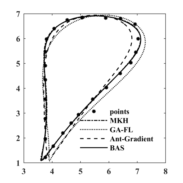
图 6.19: 各算法优化轨迹
| MKH | GA.FL | Ant.Gradient | BAS | |
|---|---|---|---|---|
| \(r_1\) | 9.99432 | 9 | 13.08 | 9.6132193 |
| \(r_2\) | 1.93027 | 3.01 | 1.89 | 1.9459840 |
| \(r_3\) | 4.57242 | 8.8 | 8.41 | 4.9080817 |
| \(r_4\) | 7.36674 | 8.8 | 6.75 | 6.6768279 |
| \(r_p\) | 8.04254 | 11.0995 | 14.45 | 8.6409226 |
| \(\theta_p\) | 0.187430 | -0.681 | 0.195 | 0.1694076 |
| \(\theta_0\) | -0.61763 | 0.489 | -0.3815 | 5.7260733 |
| \(x_0\) | -2.31301 | -2.4 | -8.77 | -2.9214626 |
| \(y_0\) | 2.86189 | -4 | 1.20 | 2.7190256 |
| \(\theta_2^1\) | * | * | * | 0.4529787 |
| \(Error\) | 0.03916 | 0.9022 | 0.5504 | 0.0397777 |