第 8 章 Python接口
项目地址 https://github.com/whhxp/Platypus 。由吴会欢同学fork Platypus项目后,修改而来。
文档内容由吴会欢同学提供。
8.1 安装方式
在线安装
还可以本地安装。
利用git 将项目克隆到本地,然后目录改为文件目录后,进行安装。
8.2 使用
Platypus是一个多目标优化库。这里我们将通过一个例子来简单介绍如何在Platypus中使用BAS。首先我们需要导入需要使用的函数
from platypus import Problem, Real
from platypus.algorithms.bas import BAS
from math import sin, pi, cos, exp, sqrt
下一步,我们需要创建问题,这里我找了三个问题作为例子。
第一个问题是Goldstein and Price problem。
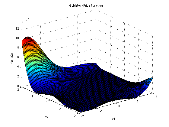
图 8.1: Goldstein-Price problem
\[\begin{equation} \begin{split} f({x})=& [1+(x_1+x_2+1)^2(19-14x_1+3x_1^2-14x_2\notag \\ & +6x_1x_2+3x_2^2)][30+(2x_1-3X_2)^2(18-32x_1\notag \\ & +12x_1^2+48x_2-36x_1x_2+27x_2^2)]\notag \end{split} \end{equation}\]
这个函数通常在正方形区间 \(x_i \in[-2,2]\)中进行评估,其中\(i = 1,2\). 全局最小值在\(x^*=(0,-1)\)处,为\(f(x^*)=3\)。
class gold(Problem):
    def __init__(self):
        super(gold, self).__init__(nvars=2, nobjs=1)
        self.types[:] = [Real(-2, 2), Real(-2, 2)]

    def evaluate(self, solution):
        vars = solution.variables[:]
        x1 = vars[0]
        x2 = vars[1]
        fact1a = (x1 + x2 + 1) ** 2
        fact1b = 19 - 14 * x1 + 3 * x1 ** 2 - 14 * x2 + 6 * x1 * x2 + 3 * x2 ** 2
        fact1 = 1 + fact1a * fact1b

        fact2a = (2 * x1 - 3 * x2) ** 2
        fact2b = 18 - 32 * x1 + 12 * x1 ** 2 + 48 * x2 - 36 * x1 * x2 + 27 * x2 ** 2
        fact2 = 30 + fact2a * fact2b
        solution.objectives[:] = [fact1 * fact2]
第一个问题是MICHALEWICZ FUNCTION。
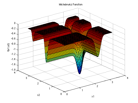
图 8.2: MICHALEWICZ FUNCTION
\[ f(x)=-\sum_{i=1}^{d}sin(x_i)[sin(\frac{ix_i^2}{\pi})]^{2m} \] Michalewicz function 有\(d!\)个局部极值,通常在\(x_i\in[0,\pi],i=1,\cdots,d\)内进行评价。
class mich(Problem):
    def __init__(self):
        super(mich, self).__init__(nvars=2, nobjs=1)
        self.types[:] = [Real(-6, -1), Real(0, 2)]

    def evaluate(self, solution):
        vars = solution.variables[:]
        x1 = vars[0]
        x2 = vars[1]
        y1 = -sin(x1) * ((sin((x1 ** 2) / pi)) ** 20)
        y2 = -sin(x2) * ((sin((2 * x2 ** 2) / pi)) ** 20)
        solution.objectives[:] = [y1 + y2]
第三个问题是ACKLEY函数(ACKLEY FUNCTION)。
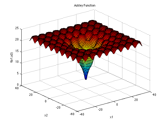
图 8.3: ACKLEY FUNCTION
\[ f(x) = -aexp(-b\sqrt{\frac{1}{d}\sum_{i=1}^dx_i^2}-exp(\frac{1}{d}\sum_{i=1}^{d}cos(cx_i))+a+exp(1) \] 推荐的测试参数为\(a=20,b=0.2,c=2\pi\), \(x_i\in[-32.768,32.768],i=1,\cdots,d\)。 全局最小值为\(f(x^*)=0,\quad at\quad x^* = (0,\cdots,0)\)
class Ackley(Problem):
    def __init__(self):
        super(Ackley, self).__init__(nvars=2, nobjs=1)
        self.types[:] = [Real(-15, 30), Real(-15, 20)]

    def evaluate(self, solution):
        vars = solution.variables[:]
        n = 2
        a = 20
        b = 0.2
        c = 2 * pi
        s1 = 0
        s2 = 0
        for i in range(n):
            s1 = s1 + vars[i] ** 2
            s2 = s2 + cos(c * vars[i])
        y = -a * exp(-b * sqrt(1 / n * s1)) - exp(1 / n * s2) + a + exp(1)
        solution.objectives[:] = [y]
然后我们将每个问题构成一个单独的实例。
接下来,我们创建BAS算法的实例。BAS算法中需要修改一些参数来获得更好的结果。例如第一个BAS实例中step=1,c=5。完成初始化后,我们可以针对不同的问题迭代不同的次数,例如第三个BAS实例中,算法迭代了300次。最后通过print函数读取最优解。可以直接输出solution这个类,他的输出顺序是:
Solution[solution.variables|solution.objectives|solution.constraints]
结果显示为:
Solution[-0.0024583254426162517,-1.002363921850713|3.0026888420039026|0]当然也可以直接输出目标函数,例如算法实例2。
结果显示为:
[-1.6524859808670134]或者也可以通过格式化的方法获得更好的输出效果
algorithm3 = BAS(problem3, step=30, c=0.1)
algorithm3.run(300)
print('Variables = {}\nObjective = {}'.format(algorithm3.best.variables,algorithm3.best.objectives))
结果显示为:
Variables = [1.52121543e-06 2.42423873e-06]
Objective = [8.095169530708546e-06]